 最新MATLAB练习题和答案.docx
- 文档编号:8189400
- 上传时间:2023-01-29
- 格式:DOCX
- 页数:34
- 大小:611.59KB
最新MATLAB练习题和答案.docx
《最新MATLAB练习题和答案.docx》由会员分享,可在线阅读,更多相关《最新MATLAB练习题和答案.docx(34页珍藏版)》请在冰豆网上搜索。
最新MATLAB练习题和答案
控制系统仿真实验
Matlab部分实验结果
实验一MATLAB基本操作
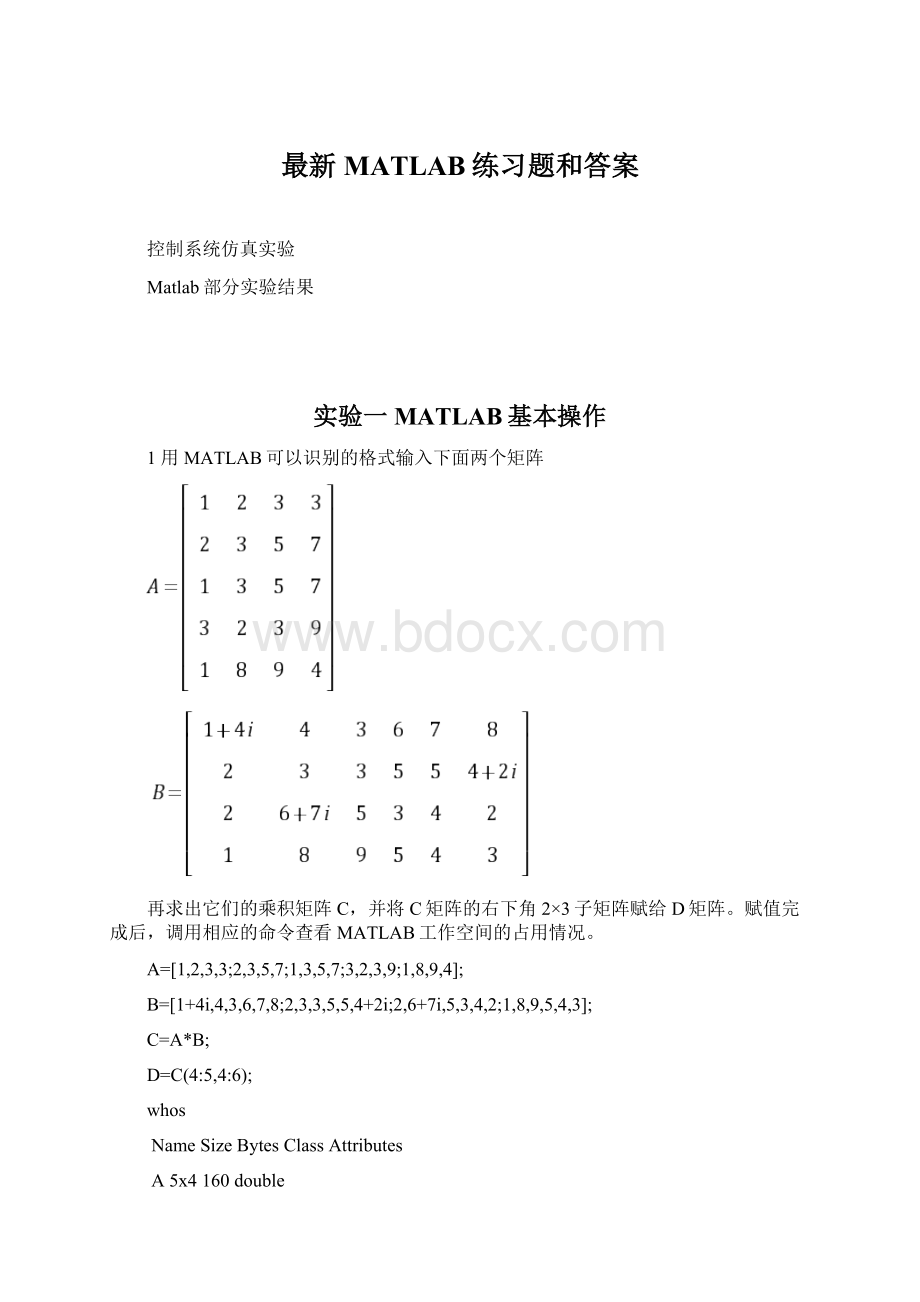
1用MATLAB可以识别的格式输入下面两个矩阵
再求出它们的乘积矩阵C,并将C矩阵的右下角2×3子矩阵赋给D矩阵。
赋值完成后,调用相应的命令查看MATLAB工作空间的占用情况。
A=[1,2,3,3;2,3,5,7;1,3,5,7;3,2,3,9;1,8,9,4];
B=[1+4i,4,3,6,7,8;2,3,3,5,5,4+2i;2,6+7i,5,3,4,2;1,8,9,5,4,3];
C=A*B;
D=C(4:
5,4:
6);
whos
NameSizeBytesClassAttributes
A5x4160double
B4x6384doublecomplex
C5x6480doublecomplex
D2x396doublecomplex
2选择合适的步距绘制出下面的图形
,其中
t=[-1:
0.1:
1];
y=sin(1./t);
plot(t,y)
3对下面给出的各个矩阵求取矩阵的行列式、秩、特征多项式、范数、特征根、特征向量和逆矩阵。
,
,
A=[7.5,3.5,0,0;8,33,4.1,0;0,9,103,-1.5;0,0,3.7,19.3];
B=[5,7,6,5;7,10,8,7;6,8,10,9;5,7,9,10];
C=[1:
4;5:
8;9:
12;13:
1rtf6];
D=[3,-3,-2,4;5,-5,1,8;11,8,5,-7;5,-1,-3,-1];
det(A);det(B);det(C);det(D);
rank(A);
rank(B);
rank(C);
rank(D);
a=poly(A);
b=poly(B);
c=poly(C);
d=poly(D);
norm(A);
norm(B);
norm(C);
norm(D);
[v,d]=eig(A,'nobalance');
[v,d]=eig(B,'nobalance');
[v,d]=eig(C,'nobalance');
[v,d]=eig(D,'nobalance');
m=inv(A);
n=inv(B);
p=inv(C);
q=inv(D);
4求解下面的线性代数方程,并验证得出的解真正满足原方程。
(a)
,(b)
(a)
A=[7,2,1,-2;9,15,3,-2;-2,-2,11,5;1,3,2,13];
B=[4;7;-1;0];
X=A\B;
C=A*X;
(b)
A=[1,3,2,13;7,2,1,-2;9,15,3,-2;-2,-2,11,5];
B=[9,0;6,4;11,7;-2,-1];
X=A\B;
C=A*X;
5.
(1)初始化一10*10矩阵,其元素均为1
ones(10,10);
(2)初始化一10*10矩阵,其元素均为0
zeros(10,10);
(3)初始化一10*10对角矩阵
v=[1:
10];
diag(v);
(4)输入A=[715;256;315],B=[111;222;333],执行下列命令,理解其含义
A(2,3)表示取A矩阵第2行、第3列的元素;
A(:
2) 表示取A矩阵的第2列全部元素;
A(3,:
)表示取A矩阵第3行的全部元素;
A(:
1:
2:
3)表示取A矩阵第1、3列的全部元素;
A(:
3).*B(:
2)表示A矩阵第3列的元素点乘B矩阵第2列的元素
A(:
3)*B(2,:
)表示A矩阵第3列的元素乘以B矩阵第2行
A*B矩阵AB相乘
A.*B矩阵A点乘矩阵B
A^2矩阵A的平方
A.^2矩阵表示求矩阵A的每一个元素的平方值
B/A表示方程AX=B的解X
B./A表示矩阵B的每一个元素点除矩阵A的元素
6在同一坐标系中绘制余弦曲线y=cos(t-0.25)和正弦曲线y=sin(t-0.5),t∈[0,2π],用不同颜色,不同线的类型予以表示,注意坐标轴的比例控制。
t=[0:
0.01:
2*pi];
y1=cos(t-0.25);
plot(t,y1,'r--')
holdon
y2=sin(t-0.5);
plot(t,y2,'k')
实验二Matlab编程
1分别用for和while循环结构编写程序,求出
并考虑一种避免循环的简洁方法来进行求和。
(a)j=1;n=0;sum=1;
forn=n+1:
63
fori=1:
n
j=j*2;
end
sum=sum+j;
j=1;
end
sum
(b)j=1;n=1;sum=1;
whilen~=64
i=1;
whilei j=j*2; i=i+1; end n=n+1; sum=sum+j; j=1; end Sum (c)i=0: 63;k=sum(2.^i); 2计算1+2+…+n<2000时的最大n值 s=0;m=0;while(s<=2000),m=m+1;s=s+m;end,m 3用MATLAB语言实现下面的分段函数 存放于文件ff.m中,令D=3,h=1求出,f(-1.5),f(0.5),f(5). D=3;h=1; x=-2*D: 1/2: 2*D; y=-h*(x<-D)+h/D./x.*((x>=-D)&(x<=D))+h*(x>D); plot(x,y); gridon f1=y(find(x==-1.5)) f2=y(find(x==0.5)) f3=y(find(x==5)) 实验三Matlab底层图形控制 1在MATLAB命令行中编程得到y=sin(t)和y1=cos(t)函数,plot(t,y);figure(10);plot(t,y1); >>t=[-pi: 0.05: pi]; >>y=sin(t); >>y1=cos(t); >>plot(t,y) >>figure(10); >>plot(t,y1) 2在MATLAB命令行中键入h=get(0),查看根屏幕的属性,h此时为根屏幕句柄的符号表示,0为根屏幕对应的标号。 >>h=get(0) h= BeingDeleted: 'off' BusyAction: 'queue' ButtonDownFcn: '' CallbackObject: [] Children: [2x1double] Clipping: 'on' CommandWindowSize: [8927] CreateFcn: '' CurrentFigure: 1 DeleteFcn: '' Diary: 'off' DiaryFile: 'diary' Echo: 'off' FixedWidthFontName: 'CourierNew' Format: 'short' FormatSpacing: 'loose' HandleVisibility: 'on' HitTest: 'on' Interruptible: 'on' Language: 'zh_cn.gbk' MonitorPositions: [111440900] More: 'off' Parent: [] PointerLocation: [1048463] PointerWindow: 0 RecursionLimit: 500 ScreenDepth: 32 ScreenPixelsPerInch: 96 ScreenSize: [111440900] Selected: 'off' SelectionHighlight: 'on' ShowHiddenHandles: 'off' Tag: '' Type: 'root' UIContextMenu: [] Units: 'pixels' UserData: [] Visible: 'on' 3h1=get (1);h2=get(10),1,10分别为两图形窗口对应标号,其中1为Matlab自动分配,标号10已在figure(10)中指定。 查看h1和h2属性,注意CurrentAxes和CurrenObject属性。 >>h1=get (1) h1= Alphamap: [1x64double] BeingDeleted: 'off' BusyAction: 'queue' ButtonDownFcn: '' Children: 170.0012 Clipping: 'on' CloseRequestFcn: 'closereq' Color: [0.80000.80000.8000] Colormap: [64x3double] CreateFcn: '' CurrentAxes: 170.0012 CurrentCharacter: '' CurrentObject: [] CurrentPoint: [00] DeleteFcn: '' DockControls: 'on' FileName: '' FixedColors: [10x3double] HandleVisibility: 'on' HitTest: 'on' IntegerHandle: 'on' Interruptible: 'on' InvertHardcopy: 'on' KeyPressFcn: '' KeyReleaseFcn: '' MenuBar: 'figure' MinColormap: 64 Name: '' NextPlot: 'add' NumberTitle: 'on' PaperOrientation: 'portrait' PaperPosition: [0.63456.345220.304615.2284] PaperPositionMode: 'manual' PaperSize: [20.984029.6774] PaperType: 'A4' PaperUnits: 'centimeters' Parent: 0 Pointer: 'arrow' PointerShapeCData: [16x16double] PointerShapeHotSpot: [11] Position: [440378560420] Renderer: 'painters' RendererMode: 'auto' Resize: 'on' ResizeFcn: '' Selected: 'off' SelectionHighlight: 'on' SelectionType: 'normal' Tag: '' ToolBar: 'auto' Type: 'figure' UIContextMenu: [] Units: 'pixels' UserData: [] Visible: 'on' WindowButtonDownFcn: '' WindowButtonMotionFcn: '' WindowButtonUpFcn: '' WindowKeyPressFcn: '' WindowKeyReleaseFcn: '' WindowScrollWheelFcn: '' WindowStyle: 'normal' WVisual: '00(RGB32GDI,Bitmap,Window)' WVisualMode: 'auto' >>h2=get(10) h2= Alphamap: [1x64double] BeingDeleted: 'off' BusyAction: 'queue' ButtonDownFcn: '' Children: 342.0011 Clipping: 'on' CloseRequestFcn: 'closereq' Color: [0.80000.80000.8000] Colormap: [64x3double] CreateFcn: '' CurrentAxes: 342.0011 CurrentCharacter: '' CurrentObject: [] CurrentPoint: [00] DeleteFcn: '' DockControls: 'on' FileName: '' FixedColors: [10x3double] HandleVisibility: 'on' HitTest: 'on' IntegerHandle: 'on' Interruptible: 'on' InvertHardcopy: 'on' KeyPressFcn: '' KeyReleaseFcn: '' MenuBar: 'figure' MinColormap: 64 Name: '' NextPlot: 'add' NumberTitle: 'on' PaperOrientation: 'portrait' PaperPosition: [0.63456.345220.304615.2284] PaperPositionMode: 'manual' PaperSize: [20.984029.6774] PaperType: 'A4' PaperUnits: 'centimeters' Parent: 0 Pointer: 'arrow' PointerShapeCData: [16x16double] PointerShapeHotSpot: [11] Position: [440378560420] Renderer: 'painters' RendererMode: 'auto' Resize: 'on' ResizeFcn: '' Selected: 'off' SelectionHighlight: 'on' SelectionType: 'normal' Tag: '' ToolBar: 'auto' Type: 'figure' UIContextMenu: [] Units: 'pixels' UserData: [] Visible: 'on' WindowButtonDownFcn: '' WindowButtonMotionFcn: '' WindowButtonUpFcn: '' WindowKeyPressFcn: '' WindowKeyReleaseFcn: '' WindowScrollWheelFcn: '' WindowStyle: 'normal' WVisual: '00(RGB32GDI,Bitmap,Window)' WVisualMode: 'auto' 4输入h.Children,观察结果。 >>h.Children ans= 1 10 5键入gcf,得到当前图像句柄的值,分析其结果与h,h1,h2中哪个一致,为什么? ans= 1 结果与h的一致 6鼠标点击Figure1窗口,让其位于前端,在命令行中键入gcf,观察此时的值,和上一步中有何不同,为什么? ans= 1 7观察h1.Children和h2.Children,gca的值。 >>h1.Children ans= 170.0012 >>h2.Children ans= 342.0011 >>gca ans= 170.0012 8观察以下程序结果h3=h1.Children;set(h3,'Color','green');h3_1=get(h3,'children');set(h3_1,'Color','red');其中h3_1为Figure1中线对象句柄,不能直接采用h3_1=h3.Children命令获得。 9命令行中键入plot(t,sin(t-pi/3)),观察曲线出现在哪个窗口。 h4=h2.Children;axes(h4);plot(t,sin(t-pi/3)),看看此时曲线显示在何窗口。 plot(t,sin(t-pi/3))后,曲线出现在figure1窗口;h4=h2.Children;axes(h4);plot(t,sin(t-pi/3))后,曲线出现在figure10 实验四控制系统古典分析 3.已知二阶系统 (1)编写程序求解系统的阶跃响应; a=sqrt(10); zeta=(1/a); num=[10]; den=[12*zeta*a10]; sys=tf(num,den); t=0: 0.01: 3; figure (1) step(sys,t);grid 修改参数,实现 和 的阶跃响应; 时: a=sqrt(10); zeta=1; num=[10]; den=[12*zeta*a10]; sys=tf(num,den); t=0: 0.01: 3; figure (1) step(sys,t);grid 时: a=sqrt(10); zeta=2; num=[10]; den=[12*zeta*a10]; sys=tf(num,den); t=0: 0.01: 3; figure (1) step(sys,t);grid 修改参数,实现 和 的阶跃响应( ) 时: a=sqrt(10); zeta=(1/a); num=[0.25]; den=[12*zeta*0.5*a0.25]; sys=tf(num,den); t=0: 0.01: 3; figure (1) step(sys,t);grid 时: a=sqrt(10); zeta=(1/a); num=[40]; den=[12*zeta*2*a40]; sys=tf(num,den); t=0: 0.01: 3; figure (1) step(sys,t);grid (2)试做出以下系统的阶跃响应,并比较与原系统响应曲线的差别与特点,作出相应的实验分析结果。 ; ; 要求: 分析系统的阻尼比和无阻尼振荡频率对系统阶跃响应的影响; 分析响应曲线的零初值、非零初值与系统模型的关系; 分析响应曲线的稳态值与系统模型的关系; 分析系统零点对阶跃响应的影响; a=sqrt(10); zeta=(1/a); num=[10]; den=[12*zeta*a10]; sys=tf(num,den); t=0: 0.01: 3; step(sys,t); holdon num1=[0210]; sys1=tf(num1,den); step(sys1,t); num2=[10.510]; sys2=tf(num2,den); step(sys2,t); num3=[10.50]; sys3=tf(num3,den); step(sys3,t); num4=[010]; sys4=tf(num4,den); step(sys4,t);grid 5 已知 令k=1作Bode图,应用频域稳定判据确定系统的稳定性,并确定使系统获得最大相位裕度的增益k值。 G=tf([11],[0.1100]); figure (1) margin(G);grid 实验五控制系统现代分析 1 (2)Bode图法判断系统稳定性: 已知两个单位负反馈系统的开环传递函数分别为: 用Bode图法判断系统闭环的稳定性。 G1=tf([2.7],[1540]); figure (1) margin(G);grid G2=tf([2.7],[15-40]); figure (2) margin(G2);grid 2 系统能控性、能观性分析 已知连续系统的传递函数模型: 当α分别取-1,0,+1时,判别系统的能控性与能观性。 当α取-1时: num=[1-1]; den=[1102718]; G=tf(num,den); G1=ss(G) a=[-10-3.375-2.25;800;010]; b=[0.5;0;0]; Uc=[b,a*b,a^2*b]; rank(Uc) a= x1x2x3 x1-10-3.375-2.25 x2800 x3010 b= u1 x10.5 x20 x30 c= x1x2x3 y100.25-0.25 d= u1 y10 Continuous-timemodel. rankUc= 3 rankUo= 3 由此,可以得到系统能控性矩阵Uc的秩是3,等于系统的维数,故系统是能控的。 能观性矩阵Uo的秩是3,等于系统的维数,故系统能观测的。 当α取0时: a= x1x2x3 x1-10-3.375-2.25 x2800 x3010 b= u1 x10.25 x20 x30 c= x1x2x3 y100.50 d= u1 y10 Continuous-timemodel. rankUc= 3 rankUo= 3 由此,可以得到系统能控性矩阵Uc的秩是3,等于系统的维数,故系统是能控的。 能观性矩阵Uo的秩是3,等于系统的维数,故系统能观测的。 当α取1时: a= x1x2x3 x1-10-3.375-2.25 x2800 x3010 b= u1 x10.5 x20 x30 c= x1x2x3 y100.250.25 d= u1 y10 rankUc= 3 rankUo= 2 由此,可以得到系统能控性矩阵Uc的秩是3,等于系统的维数,故系统是能控的。 能观性矩阵Uo的秩是2,小于系统的维数,故系统不能观测的。 实验六PID控制器的设计 1.已知三阶对象模型 ,利用MATLAB编写程序,研究闭环系统在不同控制情况下的阶跃响应,并分析结果。 (1) 时,在不同KP值下,闭环系统的阶跃响应; s=tf('s');


- 配套讲稿:
如PPT文件的首页显示word图标,表示该PPT已包含配套word讲稿。双击word图标可打开word文档。
- 特殊限制:
部分文档作品中含有的国旗、国徽等图片,仅作为作品整体效果示例展示,禁止商用。设计者仅对作品中独创性部分享有著作权。
- 关 键 词:
- 最新 MATLAB 练习题 答案
 冰豆网所有资源均是用户自行上传分享,仅供网友学习交流,未经上传用户书面授权,请勿作他用。
 对中国城市家庭的教育投资行为的理论和实证研究.docx
-
二年级下册数学练习题大全.docx
-
二十年后回故乡的优秀作文.docx
-
软基换填施工方案.docx
-
《黑白装饰画》教案.docx
-
课堂教学改革实施方案5篇.docx
-
返璞归真简约致美解读《给予树》教学设计语文.docx
-
离职证明范本精选多篇.docx
-
《天局》全文.docx
-
我害怕作文集合15篇.docx
-
伏魔战记39详细攻略.docx
-
幼儿园学期计划.docx
-
雅思分类打印版Word格式文档下载.docx
-
年产1万吨竹子纤维加工项目可行性研究报告文档格式.docx
-
电商产业化项目投资经营商业计划书Word文件下载.docx
-
医学多媒体课件的设计与制作Word文档格式.docx
-
中学生中秋节想象作文Word格式.docx
-
等保20之漏洞扫描系统技术方案建议书Word文档格式.docx
-
培训学校个人工作计划模板5篇Word格式.docx
-
北京各区二模试题分类汇编文言文阅读Word文档下载推荐.docx
-
不同职业病危害因素的防护常识Word格式文档下载.docx
-
一年级上册同音形近字练习汇总Word文档格式.docx
-
班级家长会上班主任教师讲话稿Word下载.docx
-
科斯塔环载波恢复Word文件下载.docx
-
浙教义务版六年级语文下册教案 花潮Word文件下载.docx
-
集成电路设计与集成系统专业Word格式文档下载.docx
-
开工第一课专题讲座观后感文档格式.docx
-
东城区学年第一学期高三期末化学试题及答案Word格式文档下载.docx
-
苏教版六年级语文下册第七单元测试题Word格式文档下载.docx
-
学长征精神做红色传人活动方案文档格式.docx
-
读书笔记150字30篇文档格式.docx
-
中级经济法考前必背法条精华版备考资料Word格式.docx
-
小学扶贫慰问信精选多篇Word格式.docx
-
中国科学院计算技术研究所网络与信息安全管理制度Word格式.docx
-
应届毕业生外贸跟单员实习报告Word格式.docx
-
中国科学院计算技术研究所网络与信息安全管理制度Word格式文档下载.docx
-
中考满分作文600字集锦六篇文档格式.docx
-
职业生涯规划课程设计报告及要求内容文档格式.docx
-
招教考试58题Word文档下载推荐.docx
-
多元评价促进学生全面发展.docx
-
职业生涯规划课程设计报告及要求内容Word文件下载.docx
-
小学校园生活作文Word格式文档下载.docx
-
增强共青团员意识主题教育活动问答四与增强共青团意识主题教育活动总结合集Word格式文档下载.docx
-
中国民航持续安全理念历程和主要文件共24页word资料Word文件下载.docx
-
增强共青团员意识主题教育活动问答四与增强共青团意识主题教育活动总结合集文档格式.docx
-
招教考试58题Word格式文档下载.docx
-
中国民航持续安全理念历程和主要文件共24页word资料Word文件下载.docx
-
小学一年级安全工作计划第二学期范文Word下载.docx
-
浙大宁波理工外语平台听力答案docWord文件下载.docx
-
小学语文100个常用俗语有解释有例句 2Word文档下载推荐.docx
-
中国移动重组后集团客户业务发展战略全攻略Word文档格式.docx
