 图像分割.docx
- 文档编号:5033537
- 上传时间:2022-12-12
- 格式:DOCX
- 页数:14
- 大小:1.05MB
图像分割.docx
《图像分割.docx》由会员分享,可在线阅读,更多相关《图像分割.docx(14页珍藏版)》请在冰豆网上搜索。
图像分割
这一章中主要是用数字图像处理技术对图像进行分割。
因为图像分割是个比较难的课题。
这里练习的是比较基本的。
包过点、线和边缘的检测,hough变换的应用,阈值处理,基于区域的分割以及基于分水岭方法的分割。
其练习代码和结果如下:
1%%图像分割
2
3%%点检测
4clc
5clear
6f=imread('.\images\dipum_images_ch10\Fig1002(a)(test_pattern_with_single_pixel).tif');
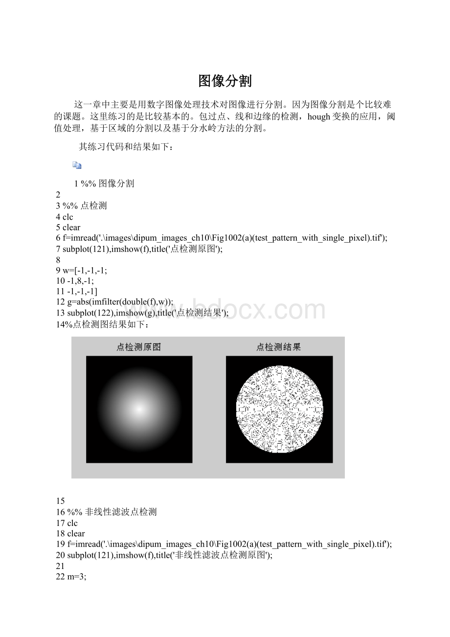
7subplot(121),imshow(f),title('点检测原图');
8
9w=[-1,-1,-1;
10-1,8,-1;
11-1,-1,-1]
12g=abs(imfilter(double(f),w));
13subplot(122),imshow(g),title('点检测结果');
14%点检测图结果如下:
15
16%%非线性滤波点检测
17clc
18clear
19f=imread('.\images\dipum_images_ch10\Fig1002(a)(test_pattern_with_single_pixel).tif');
20subplot(121),imshow(f),title('非线性滤波点检测原图');
21
22m=3;
23n=3;
24%ordfilt2(f,order,domin)表示的是用矩阵domin中为1的地方进行排序,然后选择地order个位置的值代替f中的值,属于非线性滤波
25g=imsubtract(ordfilt2(f,m*n,ones(m,n)),ordfilt2(f,1,ones(m,n)));%滤波邻域的最大值减去最小值
26T=max(g(:
));
27g2=g>=T;
28subplot(122),imshow(g2);
29title('非线性滤波点检测后图');
30%运行结果如下:
31
32%%检测指定方向的线
33clc
34clear
35f=imread('.\images\dipum_images_ch10\Fig1004(a)(wirebond_mask).tif');
36subplot(321),imshow(f);
37title('检测指定方向线的原始图像');
38
39w=[2-1-1;
40-12-1;
41-1-12];%矩阵用逗号或者空格隔开的效果是一样的
42g=imfilter(double(f),w);
43subplot(322),imshow(g,[]);
44title('使用-45度检测器处理后的图像');
45
46gtop=g(1:
120,1:
120);%取g的左上角图
47gtop=pixeldup(gtop,4);%扩大4*4倍的图
48subplot(323),imshow(gtop,[]);
49title('-45度检测后左上角放大图');
50
51gbot=g(end-119:
end,end-119:
end);%取右下角图
52gbot=pixeldup(gbot,4);%扩大16倍的图
53subplot(324),imshow(gbot,[]);
54title('-45度检测后右下角后放大图');
55
56g=abs(g);
57subplot(325),imshow(g,[]);
58title('-45度检测后的绝对值图');
59
60T=max(g(:
));
61g=g>=T;
62subplot(326),imshow(g);
63title('-45度检测后取绝对值最大的图')
64%检测指定方向的线过程如下:
65
66%%sobel检测器检测边缘
67clc
68clear
69f=imread('.\images\dipum_images_ch10\Fig1006(a)(building).tif');
70subplot(321),imshow(f);
71title('sobel检测的原始图像');
72
73[gv,t]=edge(f,'sobel','vertical');%斜线因为具有垂直分量,所以也能够被检测出来
74subplot(322),imshow(gv);
75title('sobel垂直方向检测后图像');
76
77gv=edge(f,'sobel',0.15,'vertical');
78subplot(323),imshow(gv);
79title('sobel垂直检测0.15阈值后图像');
80
81gboth=edge(f,'sobel',0.15);
82subplot(324),imshow(gboth);
83title('sobel水平垂直方向阈值0.15后图像');
84
85w45=[-2-10
86-101
87012];%相当于45度的sobel检测算子
88g45=imfilter(double(f),w45,'replicate');
89T=0.3*max(abs(g45(:
)));
90g45=g45>=T;
91subplot(325),imshow(g45);
92title('sobel正45度方向上检测图');
93
94w_45=[0-1-2
9510-1
96210];
97g_45=imfilter(double(f),w_45,'replicate');
98T=0.3*max(abs(g_45(:
)));
99g_45=g_45>=T;
100subplot(326),imshow(g_45);
101title('sobel负45度方向上检测图');
102%sobel检测过程如下:
103
104%%sobel,log,canny边缘检测器的比较
105clc
106clear
107f=imread('.\images\dipum_images_ch10\Fig1006(a)(building).tif');
108
109[g_sobel_default,ts]=edge(f,'sobel');%
110subplot(231),imshow(g_sobel_default);
111title('gsobeldefault');
112
113[g_log_default,tlog]=edge(f,'log');
114subplot(233),imshow(g_log_default);
115title('glogdefault');
116
117[g_canny_default,tc]=edge(f,'canny');
118subplot(235),imshow(g_canny_default);
119title('gcannydefault');
120
121g_sobel_best=edge(f,'sobel',0.05);
122subplot(232),imshow(g_sobel_best);
123title('gsobelbest');
124
125g_log_best=edge(f,'log',0.003,2.25);
126subplot(234),imshow(g_log_best);
127title('glogbest');
128
129g_canny_best=edge(f,'canny',[0.040.10],1.5);
130subplot(236),imshow(g_canny_best);
131title('gcannybest');
132%3者比较的结果如下:
133
134%%hough变换说明
135clc
136clear
137f=zeros(101,101);
138f(1,1)=1;
139f(101,1)=1;
140f(1,101)=1;
141f(51,51)=1;
142f(101,101)=1;
143imshow(f);title('带有5个点的二值图像');
144%显示如下:
145
146H=hough(f);
147figure,imshow(H,[]);
148title('不带标度的hough变换');
149%不带标度的hough变换结果如下:
150
151[H,theta,rho]=hough(f);
152figure,imshow(theta,rho,H,[],'notruesize');%为什么显示不出来呢
153axison,axisnormal;
154xlabel('\theta'),ylabel('\rho');
155
156%%计算全局阈值
157clc
158clear
159f=imread('.\images\dipum_images_ch10\Fig1013(a)(scanned-text-grayscale).tif');
160imshow(f);
161title('全局阈值原始图像')
162%其图片显示结果如下:
163
164T=0.5*(double(min(f(:
)))+double(max(f(:
))));
165done=false;
166while~done
167g=f>=T;
168Tnext=0.5*(mean(f(g))+mean(f(~g)));
169done=abs(T-Tnext)<0.5
170T=Tnext;
171end
172g=f<=T;%因为前景是黑色的字,所以要分离出来的话这里就要用<=.
173figure,subplot(121),imshow(g);
174title('使用迭代方法得到的阈值处理图像');
175
176
177T2=graythresh(f);%得到的是0~1的小数?
178g=f<=T2*255;
179subplot(122),imshow(g);
180title('使用函数graythresh得到的阈值处理图像');
181%阈值处理后结果如下:
182
183%%焊接空隙区域生长
184clc
185clear
186f=imread('.\images\dipum_images_ch10\Fig1014(a)(defective_weld).tif');
187subplot(221),imshow(f);
188title('焊接空隙原始图像');
189
190%函数regiongrow返回的NR为是不同区域的数目,参数SI是一副含有种子点的图像
191%TI是包含在经过连通前通过阈值测试的像素
192[g,NR,SI,TI]=regiongrow(f,255,65);%种子的像素值为255,65为阈值
193
194subplot(222),imshow(SI);
195title('焊接空隙种子点的图像');
196
197subplot(223),imshow(TI);
198title('焊接空隙所有通过阈值测试的像素');
199
200subplot(224),imshow(g);
201title('对种子点进行8连通分析后的结果');
202%焊接空隙区域生长图如下:
203
204%%使用区域分离和合并的图像分割
205clc
206clear
207f=imread('.\images\dipum_images_ch10\Fig1017(a)(cygnusloop_Xray_original).tif');
208subplot(231),imshow(f);
209title('区域分割原始图像');
210
211g32=splitmerge(f,32,@predicate);%32代表分割中允许最小的块
212subplot(232),imshow(g32);
213title('mindim为32时的分割图像');
214
215g16=splitmerge(f,16,@predicate);%32代表分割中允许最小的块
216subplot(233),imshow(g16);
217title('mindim为32时的分割图像');
218
219g8=splitmerge(f,8,@predicate);%32代表分割中允许最小的块
220subplot(234),imshow(g8);
221title('mindim为32时的分割图像');
222
223g4=splitmerge(f,4,@predicate);%32代表分割中允许最小的块
224subplot(235),imshow(g4);
225title('mindim为32时的分割图像');
226
227g2=splitmerge(f,2,@predict);%32代表分割中允许最小的块
228subplot(236),imshow(g2);
229title('mindim为32时的分割图像');
230
231%%使用距离和分水岭变换分割灰度图像
232clc
233clear
234f=imread('.\images\dipum_images_ch10\Fig0925(a)(dowels).tif');
235subplot(231),imshow(f);title('使用距离和分水岭分割原图');
236
237g=im2bw(f,graythresh(f));
238subplot(232),imshow(g),title('原图像阈值处理后的图像');
239
240gc=~g;
241subplot(233),imshow(gc),title('阈值处理后取反图像');
242
243D=bwdist(gc);
244subplot(234),imshow(D),title('使用距离变换后的图像');
245
246L=watershed(-D);
247w=L==0;
248subplot(235),imshow(w),title('距离变换后的负分水岭图像');
249
250g2=g&~w;
251subplot(236),imshow(g2),title('阈值图像与分水岭图像相与图像');
252%使用距离分水岭图像如下:
253
254%%使用梯度和分水岭变换分割灰度图像
255clc
256clear
257f=imread('.\images\dipum_images_ch10\Fig1021(a)(small-blobs).tif');
258subplot(221),imshow(f);
259title('使用梯度和分水岭变换分割灰度图像');
260
261h=fspecial('sobel');
262fd=double(f);
263g=sqrt(imfilter(fd,h,'replicate').^2+imfilter(fd,h','replicate').^2);
264subplot(222),imshow(g,[]);
265title('使用梯度和分水岭分割幅度图像');
266
267L=watershed(g);
268wr=L==0;
269subplot(223),imshow(wr);
270title('对梯度复制图像进行二值分水岭后图像');
271
272g2=imclose(imopen(g,ones(3,3)),ones(3,3));
273L2=watershed(g2);
274wr2=L2==0;
275f2=f;
276f2(wr2)=255;
277subplot(224),imshow(f2);
278title('平滑梯度图像后的分水岭变换');
279%使用梯度和分水岭变换分割灰度图像结果如下:
280
281%%控制标记符的分水岭分割
282clc
283clear
284f=imread('.\images\dipum_images_ch10\Fig1022(a)(gel-image).tif');
285imshow(f);
286title('控制标记符的分水岭分割原图像');
287
288h=fspecial('sobel');
289fd=double(f);
290g=sqrt(imfilter(fd,h,'replicate').^2+imfilter(fd,h','replicate').^2);
291L=watershed(g);
292wr=L==0;
293figure,subplot(231),imshow(wr,[]);
294title('控制标记符的分水岭分割幅度图像');
295
296rm=imregionalmin(g);%梯度图像有很多较浅的坑,造成的原因是原图像不均匀背景中灰度细小的变化
297subplot(232),imshow(rm,[]);
298title('对梯度幅度图像的局部最小区域');
299
300im=imextendedmin(f,2);%得到内部标记符
301fim=f;
302fim(im)=175;
303subplot(233),imshow(f,[]);
304title('内部标记符');
305
306Lim=watershed(bwdist(im));
307em=Lim==0;
308subplot(234),imshow(em,[]);
309title('外部标记符');
310
311g2=imimposemin(g,im|em);
312subplot(235),imshow(g2,[]);
313title('修改后的梯度幅度值');
314
315L2=watershed(g2);
316f2=f;
317f2(L2==0)=255;
318subplot(236),imshow(f2),title('最后分割的结果');
319%控制标记符的分水岭分割过程如下:


- 配套讲稿:
如PPT文件的首页显示word图标,表示该PPT已包含配套word讲稿。双击word图标可打开word文档。
- 特殊限制:
部分文档作品中含有的国旗、国徽等图片,仅作为作品整体效果示例展示,禁止商用。设计者仅对作品中独创性部分享有著作权。
- 关 键 词:
- 图像 分割
 冰豆网所有资源均是用户自行上传分享,仅供网友学习交流,未经上传用户书面授权,请勿作他用。
 如何打造酒店企业文化2刘田江doc.docx
-
律师提供著作权法律服务业务操作指引.docx
-
18秋福建师范大学《经济法》在线作业一.docx
-
施工现场危险源.docx
-
山东省潍坊市昌乐县学年七年级地理下学期期中学业质量评估试题.docx
-
新视野大学英语视听说教程第二版第一册完整答案.docx
-
精校版重庆市 初中毕业水平暨高中招生考试中考英语试题AB卷Word版含答案解析.docx
-
新视野大学英语视听说教程第二版第一册完整答案.docx
-
江苏省刘国钧中学1112学年高二语文上学期期末考前辅导试题卷苏教版会员独享.docx
-
山东省潍坊市昌乐县学年七年级地理下学期期中学业质量评估试题.docx
-
西安交通大学18年课程考试《管理会计》作业考核试题.docx
-
施工安全保证体系.docx
-
南开17秋学期《科学启蒙尔雅》在线作业2.docx
-
秋福师《大学英语1》在线作业二.docx
-
231695 北交《运输物流管理》在线作业2 15秋答案.docx
-
梁原学区安全管理工作实施方案.docx
-
环保管理台帐明细.docx
-
我国三大翻译证书考试概览.docx
-
东大17秋学期《大学英语二》在线作业31.docx
-
静态分析指标.docx
-
山东金瀚控股金瀚置业绩效考核指标库.docx
-
B0301A国际贸易.docx
-
人教版八年级数学上册同步练习试题及答案第11章《三角形》 同步练习及答案111.docx
-
秋福师《概率论》在线作业二.docx
-
17秋福师《高级英语阅读二》在线作业一.docx
-
西南大学17秋0764《工程建设监理》在线作业参考资料.docx
-
生活宝典之社会大转盘一.docx
-
专卖店管理.docx
-
100个CFO的八年之资金管理篇.docx
-
东北师范古代汉语三16秋在线作业2.docx
-
专业技术人员公共危机管理考试.docx
-
东大17秋学期《大学英语二》在线作业31.docx
-
按照传统既是食品又是中药材的物质.docx
-
北开电气区域经理行动管理办法.docx
-
会计基础知识必备.docx
-
安徽省宿州市中考物理复习专题05《热和能》.docx
-
苏教版四年级数学下册乘法运算定律练习题精选92.docx
-
十中考点1doc集美区中小学幼儿园.docx
-
基因工程知识点全.docx
-
西城外国语学校初二上期中物理.docx
-
天津监狱组织施工方案2.docx
-
PPAP生产件批准提交表单模板合集.docx
-
基础知识内部控制基本准则.docx
-
建筑工程师个人工作5总结WORD版工作总结范本供参考.docx
-
济专环境和职业健康安全管理手册修改中.docx
-
超星尔雅 朱恒源 《创新创业》期末考试.docx
-
小学政治思品教案待人宽厚教案文本.docx
-
煤制甲醇工艺原理.docx
-
百年南京浦口火车站遭废弃系朱自清《背影》发生地.docx
-
强化训练21.docx
-
完整word版运营方案.docx
