 数据挖掘如何寻找相关项.docx
- 文档编号:29235859
- 上传时间:2023-07-21
- 格式:DOCX
- 页数:11
- 大小:117.28KB
数据挖掘如何寻找相关项.docx
《数据挖掘如何寻找相关项.docx》由会员分享,可在线阅读,更多相关《数据挖掘如何寻找相关项.docx(11页珍藏版)》请在冰豆网上搜索。
数据挖掘如何寻找相关项
摘要:
我们将为您展示如何基于一个简单的公式查找相关的项目。
请注意,此项技术适用于所有的网站(如亚马逊),以个性化用户体验、提高转换效率。
查找相关项问题要想为一个特定的项目查找相关项,就必须首先为这两个项目定义相关之处。
而这些也正是你要解决的问题:
在博客上,你可能想以标签的形...
导读:
随着大数据时代浪潮的到来数据科学家这一新兴职业也越来越受到人们的关注。
本文作者AlexandruNedelcu就将数学挖掘算法与大数据有机的结合起来,并无缝的应用在面临大数据浪潮的网站之中。
数据科学家需要具备专业领域知识并研究相应的算法以分析对应的问题,而数据挖掘是其必须掌握的重要技术。
以帮助创建推动业务发展的相应大数据产品和大数据解决方案。
EMC最近的一项调查也证实了这点。
调查结果显示83%的人认为大数据浪潮所催生的新技术增加了数据科学家的需求。
本文将为您展示如何基于一个简单的公式查找相关的项目。
请注意,此项技术适用于所有的网站(如亚马逊),以个性化用户体验、提高转换效率。
查找相关项问题
要想为一个特定的项目查找相关项,就必须首先为这两个项目定义相关之处。
而这些也正是你要解决的问题:
∙在博客上,你可能想以标签的形式分享文章,或者对比查看同一个人阅读过的文章
∙亚马逊站点被称为“购买此商品的客户还购买了”的部分
∙一个类似于IMDB(InternetMovieDatabase)的服务,可以根据用户的评级,给出观影指南建议
不论是标签、购买的商品还是观看的电影,我们都要对其进行分门别类。
这里我们将采用标签的形式,因为它很简单,而且其公式也适用于更复杂的情形。
以几何关系重定义问题
现在以我的博客为例,来列举一些标签:
1.["API", "Algorithms", "Amazon", "Android", "Books", "Browser"]
好,我们来看看在欧式空间几何学中如何表示这些标签。
我们要排序或比较的每个项目在空间中以点表示,坐标值(代表一个标签)为1(标记)或者0(未标记)。
因此,如果我们已经获取了一篇标签为“API”和“Browser”的文章,那么其关联点是:
1.[ 1, 0, 0, 0, 0, 1 ]
现在这些坐标可以表示其它含义。
例如,他们可以代表用户。
如果在你的系统中有6个用户,其中2个用户对一篇文章分别评了3星和5星,那么你就可以针对此文章查看相关联的点(请注意顺序):
1.[ 0, 3, 0, 0, 5, 0 ]
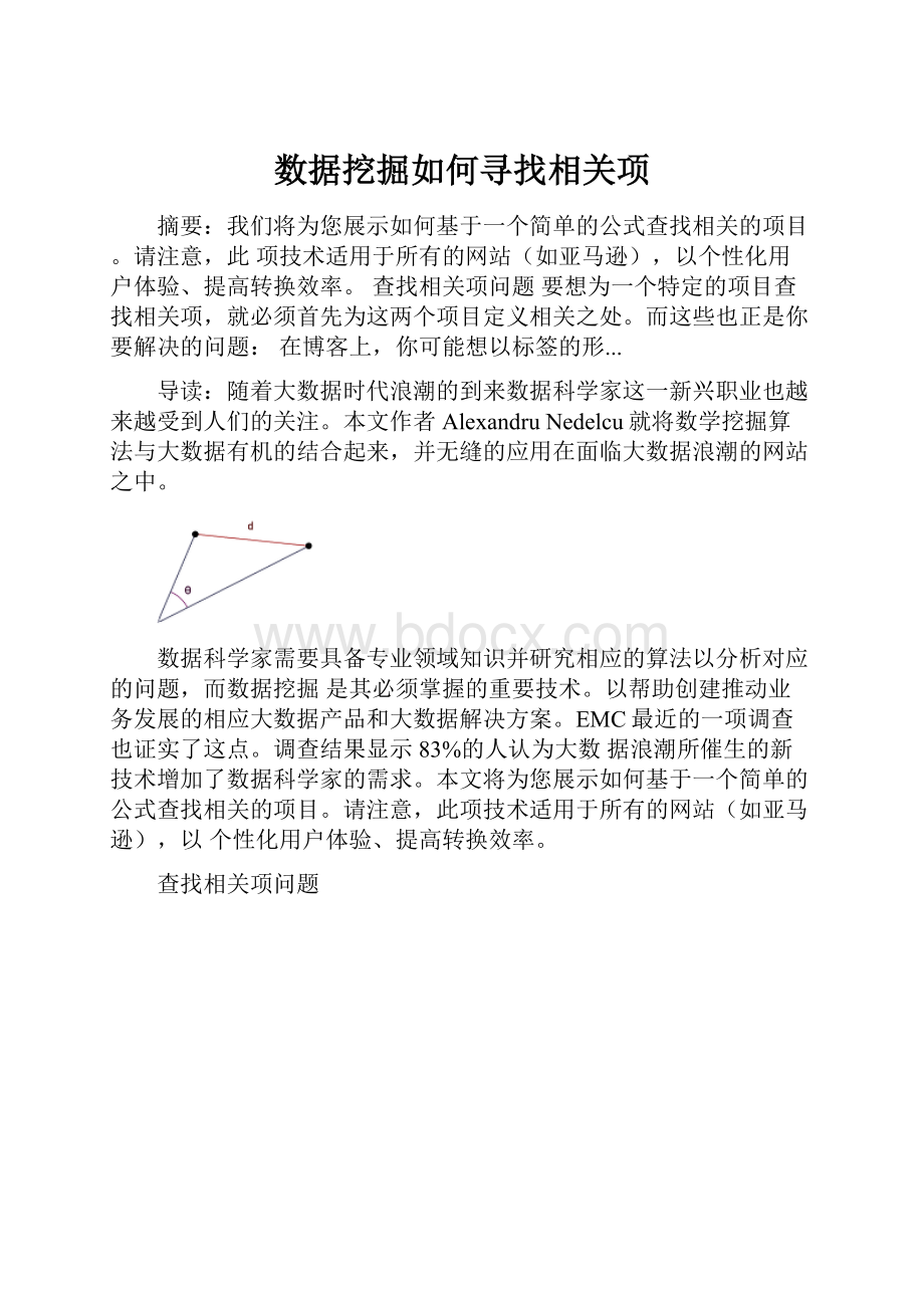
现在我们可以计算出相关矢量之间的夹角,以及这些点之间的距离。
下面是它们在二维空间中的图像:
欧式几何空间距离
计算欧式几何空间两点之间距离的数学公式非常简单。
考虑相关两点A、B之间的距离:
两点之间的距离越近,它们的相关性越大。
下面是Ruby代码:
1.# Returns the Euclidean distance between 2 points
2.#
3.# Params:
4.# - a, b:
list of coordinates (float or integer)
5.#
6.def euclidean_distance(a, b)
7. sq = a.zip(b).map{|a,b| (a - b) ** 2}
8. Math.sqrt(sq.inject(0) {|s,c| s + c})
9.end
10.# Returns the associated point of our tags_set, relative to our
11.# tags_space.
12.#
13.# Params:
14.# - tags_set:
list of tags
15.# - tags_space:
_ordered_ list of tags
16.def tags_to_point(tags_set, tags_space)
17. tags_space.map{|c| tags_set.member?
(c) ?
1 :
0}
18.end
19.# Returns other_items sorted by similarity to this_item
20.# (most relevant are first in the returned list)
21.#
22.# Params:
23.# - items:
list of hashes that have [:
tags]
24.# - by_these_tags:
list of tags to compare with
25.def sort_by_similarity(items, by_these_tags)
26. tags_space = by_these_tags + items.map{|x| x[:
tags]}
27. tags_space.flatten!
.sort!
.uniq!
28. this_point = tags_to_point(by_these_tags, tags_space)
29. other_points = items.map{|i|
30. [i, tags_to_point(i[:
tags], tags_space)]
31. }
32.
33. similarities = other_points.map{|item, that_point|
34. [item, euclidean_distance(this_point, that_point)]
35. }
36. sorted = similarities.sort {|a,b| a[1] <=> b[1]}
37. return sorted.map{|point,s| point}
38.End
这是一些示例代码,你可以直接复制运行:
1.# SAMPLE DATA
2.
3.all_articles = [
4. {
5. :
article => "Data Mining:
Finding Similar Items",
6. :
tags => ["Algorithms", "Programming", "Mining",
7. "Python", "Ruby"]
8. },
9. {
10. :
article => "Blogging Platform for Hackers",
11. :
tags => ["Publishing", "Server", "Cloud", "Heroku",
12. "Jekyll", "GAE"]
13. },
14. {
15. :
article => "UX Tip:
Don't Hurt Me On Sign-Up",
16. :
tags => ["Web", "Design", "UX"]
17. },
18. {
19. :
article => "Crawling the Android Marketplace",
20. :
tags => ["Python", "Android", "Mining",
21. "Web", "API"]
22. }
23.]
24.
25.# SORTING these articles by similarity with an article
26.# tagged with Publishing + Web + API
27.#
28.#
29.# The list is returned in this order:
30.#
31.# 1. article:
Crawling the Android Marketplace
32.# similarity:
2.0
33.#
34.# 2. article:
"UX Tip:
Don't Hurt Me On Sign-Up"
35.# similarity:
2.0
36.#
37.# 3. article:
Blogging Platform for Hackers
38.# similarity:
2.645751
39.#
40.# 4. article:
"Data Mining:
Finding Similar Items"
41.# similarity:
2.828427
42.#
43.
44.sorted = sort_by_similarity(
45. all_articles, ['Publishing', 'Web', 'API'])
46.
47.require 'yaml'
48.puts YAML.dump(sorted)
你是否留意到我们之前选择的数据存在一个缺陷?
前两篇文章对于标签“["Publishing", "Web", "API"]”有着相同的欧氏几何空间距离。
为了更加形象化,我们来看看计算第一篇文章所用到的点:
1.[1, 0, 0, 0, 0, 0, 0, 0, 0, 0, 1, 0, 0, 0, 0, 1]
2.[1, 0, 1, 0, 0, 0, 0, 0, 1, 0, 0, 1, 0, 0, 0, 1]
只有四个坐标值不同,我们再来看看第二篇文章所用到的点:
1.[1, 0, 0, 0, 0, 0, 0, 0, 0, 0, 1, 0, 0, 0, 0, 1]
2.[0, 0, 0, 0, 1, 0, 0, 0, 0, 0, 0, 0, 0, 0, 1, 1]
与第一篇文章相同,也只有4个坐标值不同。
欧氏空间距离的度量取决于点之间的差异。
这也许不太好,因为相对平均值而言,有更多或更少标签的文章会处于不利地位。
余弦相似度
这种方法与之前的方法类似,但更关注相似性。
下面是公式:
下面是Ruby代码:
1.def dot_product(a, b)
2. products = a.zip(b).map{|a, b| a * b}
3. products.inject(0) {|s,p| s + p}
4.end
5.
6.def magnitude(point)
7. squares = point.map{|x| x ** 2}
8. Math.sqrt(squares.inject(0) {|s, c| s + c})
9.end
10.
11.# Returns the cosine of the angle between the vectors
12.#associated with 2 points
13.#
14.# Params:
15.# - a, b:
list of coordinates (float or integer)
16.#
17.def cosine_similarity(a, b)
18. dot_product(a, b) / (magnitude(a) * magnitude(b))
19.end
对于以上示例,我们对文章进行分类得到:
1.- article:
Crawling the Android Marketplace
2. similarity:
0.5163977794943222
3.- article:
"UX Tip:
Don't Hurt Me On Sign-Up"
4. similarity:
0.33333333333333337
5.- article:
Blogging Platform for Hackers
6. similarity:
0.23570226039551587
7.- article:
"Data Mining:
Finding Similar Items"
8. similarity:
0.0
这种方法有了很大改善,我们的代码可以很好地运行,但它依然存在问题。
示例中的问题:
Tf-ldf权重
我们的数据很简单,可以轻松地计算并作为衡量的依据。
如果不采用余弦相似度,很可能会出现相同的结果。
Tf-ldf权重是一种解决方案。
Tf-ldf是一个静态统计量,用于权衡文本集合中的一个词在一个文档中的重要性。
根据Tf-ldff,我们可以为坐标值赋予独特的值,而并非局限于0和1.
对于我们刚才示例中的简单数据集,也许更简单的度量方法更适合,比如Jaccardindex也许会更好。
皮尔逊相关系数(Pearson Correlation Coefficient)
使用皮尔逊相关系数(Pearson Correlation Coefficient)寻找两个项目之间的相似性略显复杂,也并不是非常适用于我们的数据集合。
例如,我们在IMDB中有2个用户。
其中一个用户名为John,对五部电影做了评级:
[1,2,3,4,5]。
另一个用户名为Mary,对这五部电影也给出了评级:
[4, 5, 6, 7, 8]。
这两个用户非常相似,他们之间有一个完美的线性关系,Mary的评级都是在John的基础上加3。
计算公式如下:
代码如下:
1.def pearson_score(a, b)
2. n = a.length
3. return 0 unless n > 0
4. # summing the preferences
5. sum1 = a.inject(0) {|sum, c| sum + c}
6. sum2 = b.inject(0) {|sum, c| sum + c}
7. # summing up the squares
8. sum1_sq = a.inject(0) {|sum, c| sum + c ** 2}
9. sum2_sq = b.inject(0) {|sum, c| sum + c ** 2}
10. # summing up the product
11. prod_sum = a.zip(b).inject(0) {|sum, ab| sum + ab[0] * ab[1]}
12. # calculating the Pearson score
13. num = prod_sum - (sum1 *sum2 / n)
14. den = Math.sqrt((sum1_sq - (sum1 ** 2) / n) * (sum2_sq - (sum2 ** 2) / n))
15. return 0 if den == 0
16. return num / den
17.end
18.puts pearson_score([1,2,3,4,5], [4,5,6,7,8])
19.# => 1.0
20.puts pearson_score([1,2,3,4,5], [4,5,0,7,8])
21.# => 0.5063696835418333
22.puts pearson_score([1,2,3,4,5], [4,5,0,7,7])
23.# => 0.4338609156373132
24.puts pearson_score([1,2,3,4,5], [8,7,6,5,4])
25.# => -1
曼哈顿距离算法
没有放之四海而皆准的真理,我们所使用的公式取决于要处理的数据。
下面我们简要介绍一下曼哈顿距离算法。
曼哈顿距离算法计算两点之间的网格距离,维基百科中的图形完美诠释了它与欧氏几何距离的不同:
红线、黄线和蓝线是具有相同长度的曼哈顿距离,绿线代表欧氏几何空间距离。
(张志平/编译)


- 配套讲稿:
如PPT文件的首页显示word图标,表示该PPT已包含配套word讲稿。双击word图标可打开word文档。
- 特殊限制:
部分文档作品中含有的国旗、国徽等图片,仅作为作品整体效果示例展示,禁止商用。设计者仅对作品中独创性部分享有著作权。
- 关 键 词:
- 数据 挖掘 如何 寻找 相关
 冰豆网所有资源均是用户自行上传分享,仅供网友学习交流,未经上传用户书面授权,请勿作他用。
 《贝的故事》教案4.docx
-
《对韵歌》优秀教案8.docx
-
《函数yAsinωx+φ+P图象》wwwnet.docx
-
《静夜思》教学设计.docx
-
《汽车底盘构造与维修》题库与考核标准.docx
-
《世说新语》复习资料.docx
-
《我的服装我做主》教案设计.docx
-
《在品味情感中成长》教学片断设计.docx
-
11造价员《建设工程造价管理基础知识》精讲教程文件.docx
-
《不会叫的狗》教案 人教部编版1.docx
-
《操作系统》二学期A卷及答案.docx
-
《傅雷家书》名著阅读笔记.docx
-
《反不正当竞争法》下互联网平台封禁行为考辨以消费者用户合法权益保护为中心.docx
-
《化工原理》第六章蒸发.docx
-
《蓝海战略》概要11页.docx
-
《人生》读书心得.docx
-
《荷叶圆圆》公开课教案优秀教学设计26.docx
-
《科技出行研究报告》智能网联与新能源将变革未来汽车出行.docx
-
《272 向量的应用举例》导学案1.docx
-
《秋天》评课稿.docx
-
《电算化》第二章会计电算化的工作环境章节练习.docx
-
《室外给排水管道》施组.docx
-
《广东省建筑与装饰工程综合定额》计算规则.docx
-
《我多想去看看》教学.docx
-
《直通车车手基础认证》 考试答案 70题之欧阳育创编.docx
-
7天销量翻10倍皇冠卖家教您玩转最精准流量.docx
-
9 阿长和山海经.docx
-
《比例尺》教案.docx
-
《菜根谭》注译四闲适篇.docx
-
《福尔摩斯探案集》读后感15篇.docx
-
《红对勾》古代诗歌选择题答案补充.docx
-
《课堂密码》读后感及心得精选多篇.docx
-
11183切眼掘进工作面防突专项设计文档格式.docx
-
00医生手册免费包文档格式.docx
-
中国近代现代史复习经典单选题Word文件下载.docx
-
安徽省教师资格证考试笔试必备资料Word下载.docx
-
安徽省名校学年高三模拟联考理综化学试题及答案文档格式.docx
-
北理工激光测距实验1实验报告含代码Word文档下载推荐.docx
-
英语生日感谢信Word格式文档下载.docx
-
20XX年安检工作总结文档格式.docx
-
新人教版八年级上册英语期末复习资料Word格式文档下载.docx
-
信阳市钢材现货交易市场建设项目可行性研究报告Word文件下载.docx
-
00530中国现代文学作品选Word下载.docx
-
K12学习单元相亲相爱一家人教案1Word格式文档下载.docx
-
chap8 高等职业技术教育实践教学基地的评估Word文档格式.docx
-
学校公共卫生组织制度Word文件下载.docx
-
UT高级相关知识练习题剖析Word格式文档下载.docx
-
药品流通领域集中整治行动工作总结Word下载.docx
-
造价工程师《工程计价》真题及答案解析完美版本整理Word格式.docx
-
最新一级建造师《工程经济》最后两套密卷及答案第二套Word文件下载.docx
-
最新人教版初中物理八年级下册说课稿全集Word格式.docx
