 信号的频谱图实验报告.docx
- 文档编号:23619687
- 上传时间:2023-05-19
- 格式:DOCX
- 页数:15
- 大小:483.86KB
信号的频谱图实验报告.docx
《信号的频谱图实验报告.docx》由会员分享,可在线阅读,更多相关《信号的频谱图实验报告.docx(15页珍藏版)》请在冰豆网上搜索。
信号的频谱图实验报告
大连理工大学实验报告
学院(系):
专业:
______________________班级:
___
姓名:
学号:
组:
___
实验时间:
实验室:
实验台:
指导教师签字:
成绩:
实验一信号的频谱图
一、实验目的
1.掌握周期信号的傅里叶级数展开
2.掌握周期信号的有限项傅里叶级数逼近
3.掌握周期信号的频谱分析
4.掌握连续非周期信号的傅立叶变换
5.掌握傅立叶变换的性质
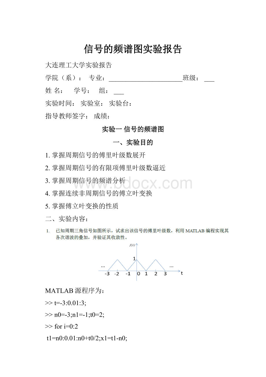
二、实验内容:
MATLAB源程序为:
>>t=-3:
0.01:
3;
>>n0=-3;n1=-1;t0=2;
>>fori=0:
2
t1=n0:
0.01:
n0+t0/2;x1=t1-n0;
t2=n1-t0/2:
0.01:
n1;x2=-t2+n1;
plot(t1,x1,'r',t2,x2,'r');
holdon;
n0=n0+t0;n1=n1+t0;
end
>>n_max=[1371531];
>>N=length(n_max);
>>fork=1:
N
n=1;sum=0;
while(n<(n_max(k)+1))
b=4./pi/pi/n/n;
y=b*cos(n*pi*t);
sum=sum+y;
n=n+2;
end
figure;
n0=-3;n1=-1;t0=2;
fori=0:
2
t1=n0:
0.01:
n0+t0/2;x1=t1-n0;
t2=n1-t0/2:
0.01:
n1;x2=-t2+n1;
plot(t1,x1,'r',t2,x2,'r');
holdon;
n0=n0+t0;n1=n1+t0;
end
y=sum+0.5;
plot(t,y,'b');
xlabel('t'),ylabel('wove');
holdoff;
axis([-3.013.01-0.011.01]);
gridon;
title(['themax=',num2str(n_max(k))])
end
运行结果:
MATLAB源程序为:
>>fork=1:
3;
n=-30:
30;tao=k;T=2*k;w=2*pi/T;
x=n*tao*0.5
fn1=sinc(x/pi);
fn=tao*fn1.*fn1;
subplot(3,1,k),stem(n*w,fn);
gridon
title(['T=',num2str(2*k)]);
axis([-30300k]);
end
运行结果:
x=
Columns1through9
-15.0000-14.5000-14.0000-13.5000-13.0000-12.5000-12.0000-11.5000-11.0000
Columns10through18
-10.5000-10.0000-9.5000-9.0000-8.5000-8.0000-7.5000-7.0000-6.5000
Columns19through27
-6.0000-5.5000-5.0000-4.5000-4.0000-3.5000-3.0000-2.5000-2.0000
Columns28through36
-1.5000-1.0000-0.500000.50001.00001.50002.00002.5000
Columns37through45
3.00003.50004.00004.50005.00005.50006.00006.50007.0000
Columns46through54
7.50008.00008.50009.00009.500010.000010.500011.000011.5000
Columns55through61
12.000012.500013.000013.500014.000014.500015.0000
x=
Columns1through16
-30-29-28-27-26-25-24-23-22-21-20-19-18-17-16-15
Columns17through32
-14-13-12-11-10-9-8-7-6-5-4-3-2-101
Columns33through48
234567891011121314151617
Columns49through61
18192021222324252627282930
x=
Columns1through9
-45.0000-43.5000-42.0000-40.5000-39.0000-37.5000-36.0000-34.5000-33.0000
Columns10through18
-31.5000-30.0000-28.5000-27.0000-25.5000-24.0000-22.5000-21.0000-19.5000
Columns19through27
-18.0000-16.5000-15.0000-13.5000-12.0000-10.5000-9.0000-7.5000-6.0000
Columns28through36
-4.5000-3.0000-1.500001.50003.00004.50006.00007.5000
Columns37through45
9.000010.500012.000013.500015.000016.500018.000019.500021.0000
Columns46through54
22.500024.000025.500027.000028.500030.000031.500033.000034.5000
Columns55through61
36.000037.500039.000040.500042.000043.500045.0000
MATLAB源程序为:
(1)>>ft=sym('sin(2*pi*(t-1))/(pi*(t-1))');
>>Fw=fourier(ft);
>>subplot(2,1,1);
>>ezplot(abs(Fw));
>>gridon;
>>title('fudupu');
>>phase=atan(imag(Fw)/real(Fw));
>>subplot(2,1,2);
>>ezplot(phase);
>>gridon;
>>title('xiangweipu');
运行结果:
(2)
MATLAB源程序为:
>>ft=sym('(sin(pi*t)/(pi*t))^2');
>>Fw=fourier(ft);
>>subplot(2,1,1);
>>ezplot(abs(Fw));
>>gridon;
>>title('fudupu');
>>phase=atan(imag(Fw)/real(Fw));
>>subplot(2,1,2);
>>ezplot(phase);
>>gridon;
>>title('xiangweipu');
运行结果:
(1)
MATLAB源程序为:
>>symst
>>Fw=sym('10/(3+i*w)-4/(5+i*w)')
Fw=
10/(w*i+3)-4/(w*i+5)
>>ft=ifourier(Fw,t)
ft=
(20*pi*exp(-3*t)*heaviside(t)-8*pi*exp(-5*t)*heaviside(t))/(2*pi)
>>ezplot(ft);
>>gridon;
运行结果:
(2)
MATLAB源程序为:
>>symst
>>Fw=sym('exp(-4*w^2)')
Fw=
exp(-4*w^2)
>>ft=ifourier(Fw,t)
ft=
exp(-t^2/16)/(4*pi^(1/2))
>>ezplot(ft);
>>gridon;
运行结果:
MATLAB源程序为:
>>dt=0.01;
>>t=-4:
dt:
4;
>>gt=(-1/2<=t&t<=1/2);
>>N=2000;
>>k=-N:
N;
>>W=2*pi*k/((2*N+1)*dt);
>>F=dt*gt*exp(-j*t'*W);
>>plot(W,F);
警告:
复数X和/或Y参数的虚部已忽略
>>gridon
>>xlabel('W'),ylabel('F(W)')
>>title('频谱图');
>>axis([-200200-0.251.1]);
运行结果:
MATLAB源程序为:
>>dt=0.01;
>>t=-0.6:
dt:
0.6;
>>f=rectpuls(t,1);
>>F=conv(f,f)*dt;n=length(F);
>>tt=(0:
n-1)*dt-1.2;
>>N=2000;k=-N:
N;
>>w=2*pi*k/((2*N+1)*dt);
>>fw=dt*f*exp(-j*t'*w);
>>FW=dt*F*exp(-j*tt'*w);
>>subplot(321),plot(t,f,'linewidth',2),gridon;
>>axis([-0.7,0.7,-0.1,1.1]);
>>title('f');%门信号图形
>>subplot(322),plot(w,fw,'linewidth',2),gridon;
警告:
复数X和/或Y参数的虚部已忽略
>>axis([-20,20,-0.5,1.1]);
>>title('fw');%门信号频谱图
>>subplot(323),plot(tt,F,'linewidth',2),gridon;
>>axis([-1.3,1.3,-0.2,1.2]);
>>title('f*f');%两门信号卷积的图形
>>subplot(324),plot(w,fw.*fw,'linewidth',2),gridon;
警告:
复数X和/或Y参数的虚部已忽略
>>axis([-20,20,-0.1,1.1]);
>>title('fw*fw');%门信号频域相乘的图形
>>subplot(326),plot(w,FW,'linewidth',2),gridon;
警告:
复数X和/或Y参数的虚部已忽略
>>axis([-20,20,-0.1,1.1]);
>>title('Fourier(f*f)');%两门信号卷积,再Fourier变换
>>
运行结果:
由于两门信号卷积的图形与两门信号卷积再傅里叶变换的图形基本一致,所以傅里叶变换的时域卷积定理得证。
三、实验体会
这是第一次信号上机实验,在这次实验中第一次接触到了MATLAB这个工程软件,MATLAB功能强大,操作相对简单。
同时本节课中我学会了对绘制信号的时域波形和对信号进行频域分析。
通过MATLAB可以非常直观的看到了,信号的叠加合成等现象。


- 配套讲稿:
如PPT文件的首页显示word图标,表示该PPT已包含配套word讲稿。双击word图标可打开word文档。
- 特殊限制:
部分文档作品中含有的国旗、国徽等图片,仅作为作品整体效果示例展示,禁止商用。设计者仅对作品中独创性部分享有著作权。
- 关 键 词:
- 信号 频谱 实验 报告
 冰豆网所有资源均是用户自行上传分享,仅供网友学习交流,未经上传用户书面授权,请勿作他用。
 《酒店人力资源管理》教案.docx
-
《马克思主义基本原理概论》选择题复习题.docx
-
《全国100所名校示范卷》高三生物人教版西部卷一轮复习 第十五单元 《稳态与环境》综合检测.docx
-
《1吨有多重》教学设计反思及评点2篇.docx
-
《红飘带狮王》读书笔记.docx
-
《教综》真题答案.docx
-
《企业管理》复习题发学生.docx
-
《提高数学学困生的学习兴趣研究》课题工作总结报告.docx
-
《蟋蟀的住宅》的教学设计.docx
-
《园林建筑设计》教案.docx
-
《中西医结合内科学》精华笔记.docx
-
2三轴向加速度传感器长春汽车工业高等专科学校.docx
-
04装修工程施工合同.docx
-
5套打包四年级数学上期中考试单元综合练习题含答案解析.docx
-
《食品安全法》知识竞赛题目及答案.docx
-
《24式简化太极拳》简案.docx
-
《金融理论与实务》复习大纲.docx
-
《旅游地理》学案.docx
-
《企业集团财务管理》综合练习题参考答案11春.docx
-
《实践论》原文毛泽东.docx
-
《项目管理软件》课程复习题.docx
-
《员工手册》电子版范文.docx
-
《中小学布局整改措施》.docx
-
5旋风分离器安装.docx
-
10kV跨越架搭设施工方案设计.docx
-
#市关爱儿童服务中心暨救助站改造工程项目建议书.docx
-
《毛概》课程标准.docx
-
《人民日报》学习贯彻党的十七届四中全会精神系列.docx
-
《我的军训生活》作文800字.docx
-
《研发人员绩效考核奖励办法》.docx
-
1 《道路交通安全法》规定任何单位或者个人不得收缴机.docx
-
02电气检修规程.docx
-
朱震字子发荆门军人阅读理解与答案解析.docx
-
住院病历书写规范及范例.docx
-
注会财管题 40.docx
-
专业工程分包管理办法.docx
-
装备制造业产业集群述评 区域经济陆媛媛.docx
-
资产负债表分析习题汇总.docx
-
资金监管协议.docx
-
自动扶梯安装工艺.docx
-
自考《幼儿园课程》内部资料白皮书题库.docx
-
自制杨梅干分析.docx
-
综合单价分析表.docx
-
足球俱乐部创业计划书.docx
-
最全六级的范文50篇经典版doc.docx
-
最新初一上册英语单词听写用复习课程.docx
-
最新高考近义成语辨析题训练.docx
-
一年级的教学工作计划.docx
-
一年级数学下册100以内连加连减口算题讲课教案.docx
-
医疗器械现场检查原则.docx
-
医院门诊系统设计说明书.docx
