 基于Matlab的数字信号传输系统实验.docx
- 文档编号:125006
- 上传时间:2022-10-04
- 格式:DOCX
- 页数:3
- 大小:303.94KB
基于Matlab的数字信号传输系统实验.docx
《基于Matlab的数字信号传输系统实验.docx》由会员分享,可在线阅读,更多相关《基于Matlab的数字信号传输系统实验.docx(3页珍藏版)》请在冰豆网上搜索。
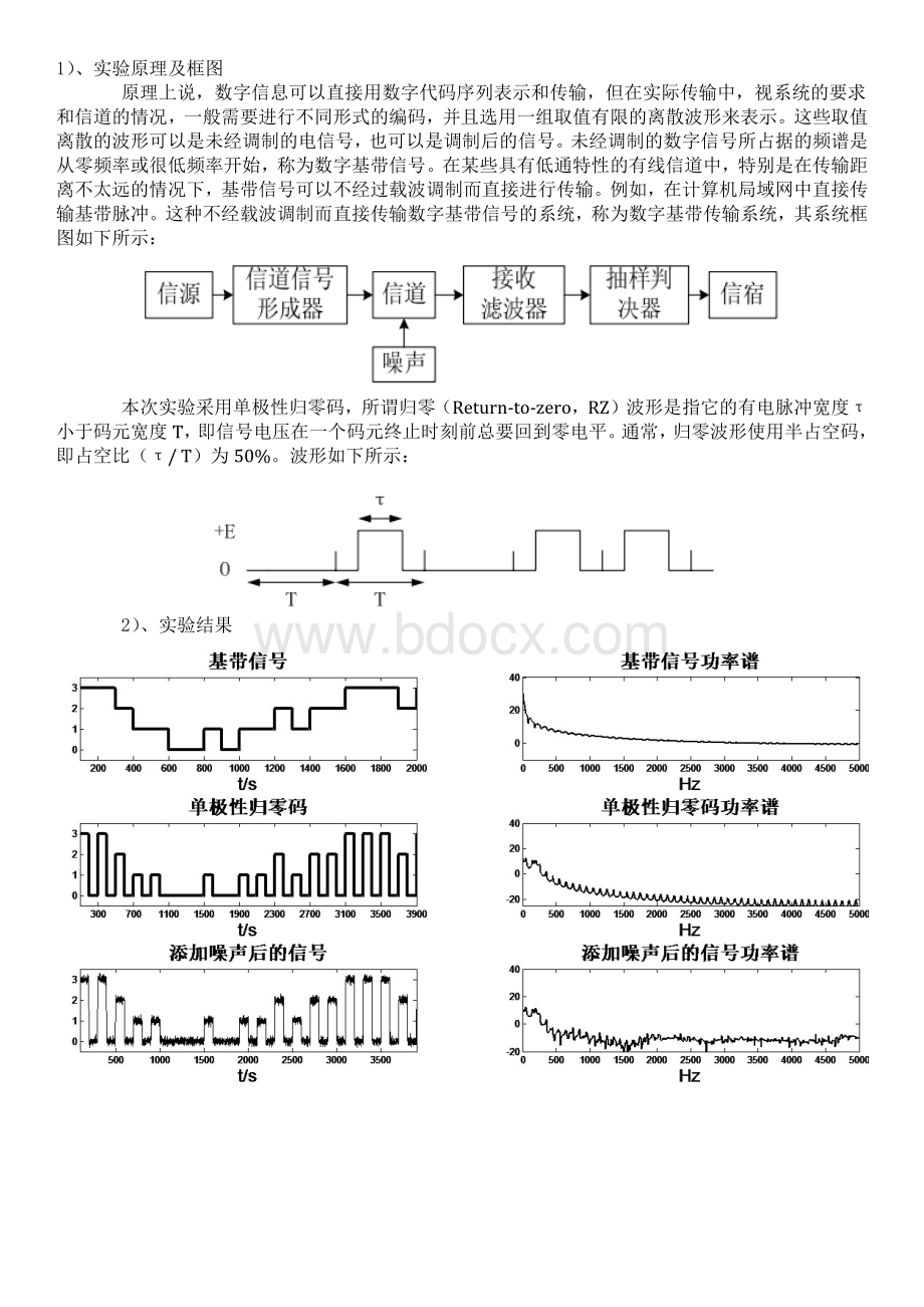
1)、实验原理及框图
原理上说,数字信息可以直接用数字代码序列表示和传输,但在实际传输中,视系统的要求和信道的情况,一般需要进行不同形式的编码,并且选用一组取值有限的离散波形来表示。
这些取值离散的波形可以是未经调制的电信号,也可以是调制后的信号。
未经调制的数字信号所占据的频谱是从零频率或很低频率开始,称为数字基带信号。
在某些具有低通特性的有线信道中,特别是在传输距离不太远的情况下,基带信号可以不经过载波调制而直接进行传输。
例如,在计算机局域网中直接传输基带脉冲。
这种不经载波调制而直接传输数字基带信号的系统,称为数字基带传输系统,其系统框图如下所示:
本次实验采用单极性归零码,所谓归零(Return-to-zero,RZ)波形是指它的有电脉冲宽度τ小于码元宽度T,即信号电压在一个码元终止时刻前总要回到零电平。
通常,归零波形使用半占空码,即占空比(τ/T)为50%。
波形如下所示:
2)、实验结果
附:
程序源代码
Fs=1e4; %采样频率
len=20; %码元长度
in=randint(1,len,4); %产生初始码元序列
sig=[];
out=[];
fort=1:
2000 %产生基带信号
n=fix(t/100);
ifn==0
in_a(t)=0;
else
in_a(t)=in(n);
end
end
subplot(2,1,1); %基带信号
plot(in_a,'LineWidth',3);
title('基带信号','FontWeight','bold','FontSize',20);
xlabel('t/s','FontSize',18);
axis([100,2100,-0.5,3.5]);
set(gca,'XTick',0:
100:
2000);
gridon;
cxn=xcorr(in_a,'unbiased');%%计算序列的自相关函数
nfft=1024;
CXk=fft(cxn,nfft);
Pxx=abs(CXk);
index=0:
round(nfft/2-1);
k=index*Fs/nfft;
subplot(2,1,2);
plot_Pxx=10*log10(Pxx(index+1));
plot(k,plot_Pxx,'LineWidth',2);
title('基带信号功率谱','FontWeight','bold','FontSize',20);
axis([0,5000,-10,40]);
xlabel('Hz','FontSize',18,'FontSize',18);
fori=1:
len%产生单极性归零码信号
ifin(i)==0
ins=[0,0];
elseifin(i)==1
ins=[1,0];
elseifin(i)==2
ins=[2,0];
else
ins=[3,0];
end
sig=[sig,ins];
end
fort=1:
4000
n=fix(t/100);
ifn==0
s(t)=0;
else
s(t)=sig(n);
end
end
figure;
subplot(2,1,1);%单极性归零码
plot(s,'LineWidth',3);
title('单极性归零码','FontWeight','bold','FontSize',20);
xlabel('t/s','FontSize',18);
axis([100,4100,-0.5,3.5]);
set(gca,'XTick',0:
200:
4100);
gridon;
cxn=xcorr(s,'unbiased');
nfft=1024;
CXk=fft(cxn,nfft);
Pxx=abs(CXk);
index=0:
round(nfft/2-1);
k=index*Fs/nfft;
subplot(2,1,2);
plot_Pxx=10*log10(Pxx(index+1));
plot(k,plot_Pxx,'LineWidth',2);
title('单极性归零码功率谱','FontWeight','bold','FontSize',20);
axis([0,5000,-10,40]);
xlabel('Hz','FontSize',18);
s1=awgn(s,20);%添加噪声
figure;
subplot(2,1,1);
plot(s1);
title('添加噪声后的信号','FontWeight','bold','FontSize',20);
xlabel('t/s','FontSize',18);
axis([100,4100,-0.5,3.5]);
set(gca,'XTick',0:
500:
4100);
cxn=xcorr(s1,'unbiased');
nfft=1024;
CXk=fft(cxn,nfft);
Pxx=abs(CXk);
index=0:
round(nfft/2-1);
k=index*Fs/nfft;
subplot(2,1,2);
plot_Pxx=10*log10(Pxx(index+1));
plot(k,plot_Pxx,'LineWidth',2);
title('添加噪声后的信号功率谱','FontWeight','bold','FontSize',20);
axis([0,5000,-10,40]);
xlabel('Hz','FontSize',18); %滤波器设计
fp=500; %通带截止
fs=550; %阻带截止
ws=fs*2/Fs;
wp=fp*2/Fs;
[N,Wp]=ellipord(wp,ws,1,40);
[b,a]=ellip(N,1,40,Wp);
sf0=filter(b,a,s1);%滤掉部分噪声后的信号
figure;
subplot(2,1,1);
plot(sf0);
title('滤掉部分噪声后的信号','FontWeight','bold','FontSize',20);
xlabel('t/s','FontSize',18);
set(gca,'XTick',0:
500:
4100);
cxn=xcorr(sf0,'unbiased');nfft=1024;
CXk=fft(cxn,nfft);
Pxx=abs(CXk);
index=0:
round(nfft/2-1);
k=index*Fs/nfft;
subplot(2,1,2);
plot_Pxx=10*log10(Pxx(index+1));
plot(k,plot_Pxx,'LineWidth',2);
title('滤掉部分噪声后的信号功率谱','FontWeight','bold','FontSize',20);
axis([0,5000,-10,40]);
xlabel('Hz','FontSize',18,'FontSize',18);
form=1:
20%抽样判决
p=round(sf0(200*m-20));
out=[out,p];
end
figure;
subplot(2,1,1);%原始码元序列
stairs(in,'LineWidth',3);
title('原始码元序列','FontWeight','bold','FontSize',20);
axis([1,21,-0.5,3.5]);
set(gca,'XTick',0:
1:
20);
gridon;
subplot(2,1,2);%抽样判决后恢复的信号序列
stairs(out,'LineWidth',3);
title('抽样判决后恢复的信号序列','FontWeight','bold','FontSize',20);
axis([1,21,-0.5,3.5]);
set(gca,'XTick',0:
1:
20);
gridon;


- 配套讲稿:
如PPT文件的首页显示word图标,表示该PPT已包含配套word讲稿。双击word图标可打开word文档。
- 特殊限制:
部分文档作品中含有的国旗、国徽等图片,仅作为作品整体效果示例展示,禁止商用。设计者仅对作品中独创性部分享有著作权。
- 关 键 词:
- 基于 Matlab 数字信号 传输 系统 实验
 冰豆网所有资源均是用户自行上传分享,仅供网友学习交流,未经上传用户书面授权,请勿作他用。
 第二章-传统相机的性能与种类.ppt
 三级健康管理师题库(附答案).docx
-
房屋租赁合同范本(有法律效益).docx
-
合作协议书中(英文)版.docx
-
人音版小学三年级上册音乐教案.docx
-
餐饮店合股投资协议书.docx
-
城市综合管廊特点及设计要点解析.docx
-
机械助理工程师个人工作总结.docx
-
建设单位会议管理办法.docx
-
国有企业在“一带一路”中的发展路径.docx
-
幼儿园与家长签订的安全责任书.docx
-
2018年助理值班员职业技能竞赛专业知识考试试题及答案.docx
-
初中物理学科的核心素养.docx
-
军训结束教官讲话稿范本.docx
-
人教版新起点五年级英语上册全册教案.docx
-
唱歌跑调怎样办,唱歌超难听怎样办.docx
-
某拟提拔干部近三年工作总结.docx
-
最美教师事迹材料.docx
-
广播电视概论第一章绪论.pptx
-
质量管理体系考试试题及答案2.docx
-
《串联和并联》练习题.pptx
-
高端装备制造项目可行性研究报告.docx
-
新教师入职培训心得体会(9篇).docx
-
最新部编版三年级上册语文第8课《卖火柴的小女孩》教案第3单元教学设计.docx
-
2019年初级保育员理论知识考试真题及答案.docx
 专业分包合同风险控制要点一览表 - 副本.rtf
-
2019年最新主题教育围绕“四个对照”“四个找一找”在专题民主(组织)生活会个人对照检视检查研讨材料.docx
-
2018年度公司培训计划方案.docx
-
企业债券发行法律服务意向书---律所整理.docx
-
2019年事业单位法律知识考题及答案解析.docx
-
2019-2020学年人教版(新起点)英语五年级上册全册教案.docx
-
轨道焊接方案.docx
-
国家公务员行测申论真题及其答案.docx
-
河南省鹤壁市高级中学学年高三第四次模拟英语试题 Word版含答案.docx
-
电工实训报告总结.docx
-
电磁感应电涡流.docx
-
当前的形势与领导者的素质.docx
-
河北出入境检验检疫局数据中心维修维护服务项目需求.docx
-
国赛中职组ZZ028 电子电路装调与应用赛项规程.docx
-
各级各部门安全生产责任制考核办法.docx
-
导读《昆虫记》知识点梳理.docx
-
读书的乐趣作文18篇.docx
-
国营企业劳动合同范本.docx
-
道路运输车辆管理二级维护新规定.docx
-
国外水泥工业英语词汇大全.docx
-
给学院的建议书范文汇总10篇.docx
-
海南省建设工程造价管理办法.docx
-
灯具安装施工方案.docx
-
多塔作业安全专项方案.docx
-
汉语言文学浅析李清照词风的阶段性变化.docx
-
第4届运动会秩序册.docx
